

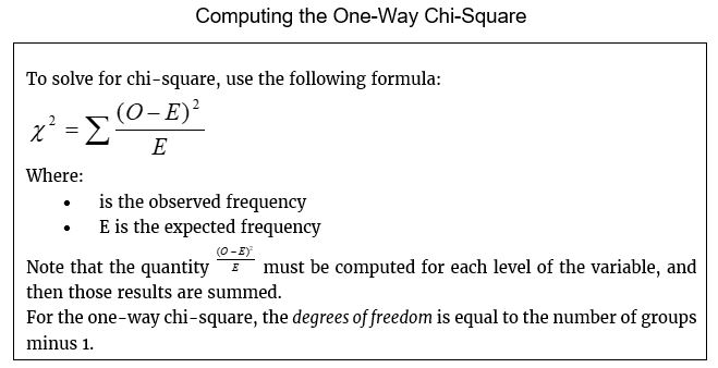
Whereas the t and F tests we have previously discussed examine the differences between means, chi-square is a test of the difference between frequencies. This test is also identified by its Greek letter designation, χ2. The null hypothesis for the chi-square test asserts that the observed differences in frequencies were a result of sampling error. Like the other significance tests we have discussed, the null hypothesis is rejected when the probability of the null hypothesis being true is low, such as p < .05 or p < .01. It is important to note that when the frequencies are statistically different, then the percentages based on those frequencies are also statistically different.
The way the chi-square test works is relatively simple. Rather than comparing means, we compare observed frequencies with expected frequencies. Observed frequencies are the result of our experimental observations. Expected frequencies are the values that we would expect of the null hypothesis was true. These are usually expressed as O and E in the formulas. Often, the expected frequencies are the total sample split into even groups. For example, if we have a variable with four possible conditions, we could assume that if there were no differences in frequencies, then 25% of the subjects would fall into each group. Anything that differs from 25% suggests that the null hypothesis may be false.
This strategy does not make sense all the time, such as when theory suggests that the groups should be of different sizes. Let us say we are interested in the variable gender in retirement community residents. It would be imprecise to set the expected frequencies at 50% male and 50% female because we know that among the elderly, women are represented in higher numbers because they have a longer life expectancy than men do.
Like the ANOVA designed we discussed in earlier chapters, chi-square tests can be thought of as having ways (synonymous with factors in parametric tests). When one variable with several levels is being compared (such as political party with the possible values of Democrat, Republican, and Independent), the test can be considered a one-way test.
Note that when we refer to the variable being analyzed with a chi-square test, we are usually referring to a grouping variables measured at the nominal level. What we are generally measuring is how many individuals fall into a particular group. Unlike with mean difference tests, you will never see a table of means and standard deviations reported with a chi-square test because these statistics are inappropriate given the measurement level of the data.
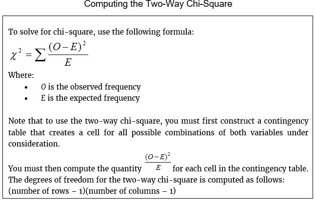
With the two-way chi-square, we are looking are defining group membership using two categories. When we put this into a table, it is often referred to as a contingency table. A contingency table is a statistical table that classifies subjects according to two nominal (grouping) variables with columns representing one variable and rows representing another variable. To confuse matters further, contingency tables are also called cross-tabulations or crosstabs. Discussions about chi-square results often refer to cells and cell values. This is because there is a cell and a frequency for that cell for each possible combination of variables.
Let us say for example a researcher is interested in the relationship between support for the death penalty and gender. Here we have two variables, each with two levels. We can arrange those into a simple table:

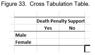

The table above represents the simplest form of two-way chi-square. Since each variable (support for the death penalty and gender) has two levels, this can be referred to as a 2 x 2 contingency table.
In a research situation where there is not a reason to assume that cell frequencies will be equally divided, we can compute an expected frequency based on the assumption that the frequency for one variable should be evenly split across the other variable. In our death penalty example, we have no idea how many people we should expect to support the death penalty. However, if there were no relationship between death penalty support and gender, we would expect both genders to have the same frequency.

Note that the magnitude of chi-square is directly related to how big the difference between the observed frequency and the expected frequency is. The larger the value of chi-square, the more likely we are to have statistically significant results. This stands to reason since the bigger the difference between the categories, the more comfortable we are saying that there are real differences and we did not get those results by sampling error. From this, we can see that a large difference between the observed and expected frequencies increases the power of a particular test, just as a large difference between means increases the power of t and F tests.
The accuracy of chi-square depends on how well the probability of the calculated value of chi-square is described by the chi-square distribution. In other words, the sampling distribution does not fit the table values we use to reject the null hypothesis. The smaller the sample size, the worse the fit. While there is some disagreement among statisticians, a common rule of thumb is not to use chi-square if one or more of the expected frequencies falls below five. We can flip this to say that it is a basic assumption of the chi-square test that the expected frequency of all cells has a value above five.
Last Modified: 06/04/2021