
To the student experienced with computing t-tests by hand, the method that is used in Excel seems somewhat backward. The trick is to compute the probability, then you get the inverse of the probability to determine the value of t.
The first step is to place your data into columns, taking care to keep X1 and X2 paired. The next step is to compute the probability associated with the t statistic using the TTEST function. Examine the dialog box for this function below:
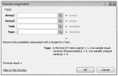
Note the help text for “Type” at the bottom of the box. To choose which type of t-test you want the probability reported for, select the appropriate number. Since we are working with dependent data, we enter 1 for “paired.” For tails, enter 2 to let Excel know that we are conducting a two-tailed test. Array1 is the block of cells that contain the values for X1, and Array2 is the block of cells that contain the values for X2.
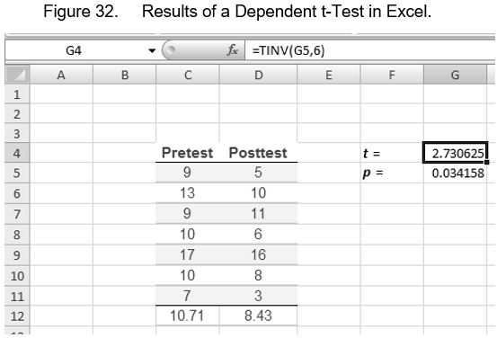
Note the results in Figure 32 below. The value of t is computed using the TINV function, which produces the inverse value of a probability of t. This is a fancy way of saying that given the probability of t, it gives you t. Note the number 6 in the function box as the last argument for the TINV function. It represents the degrees of freedom, N – 1.
Key Terms
t-Test, Independent Group, t-Test for Independent Groups, Dependent Groups, Matching, Correlated Data, Paired Data
Last Modified: 06/04/2021